强化学习的数学原理-第8课

2025年12月23日

20:37

Value Function Approximation

(from tabular representation to function representation)

 

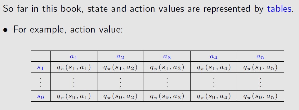
表格表示的好处有：intuitive并且容易分析

缺点有：当状态很多时，或状态是连续的变量时，需要存储很多值，并且泛化性差（因为很难访问到

全部的状态）

 

如下图所示，假设v(s)的分布点如下，我们希望用曲线或直线对v(s)进行拟合，

 

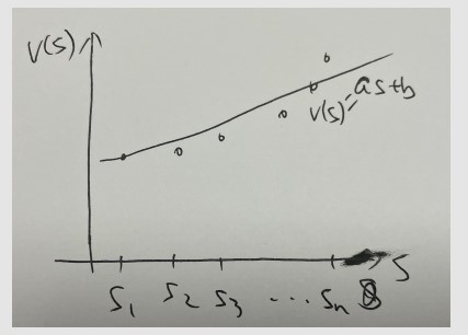
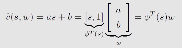
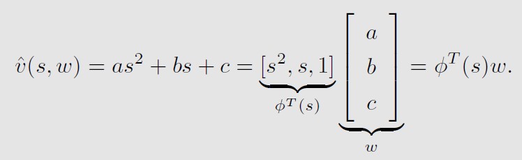
假设用一条直线来拟合，可以写成如下的形式，

也可以用更高阶的函数来拟合，

 

 

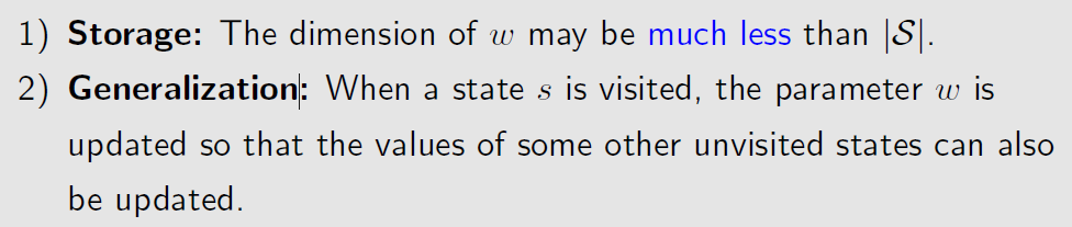
用函数代表表格的好处：

 

总结一下，现在是要用v_hat(s,w)来估计v(s)，

 

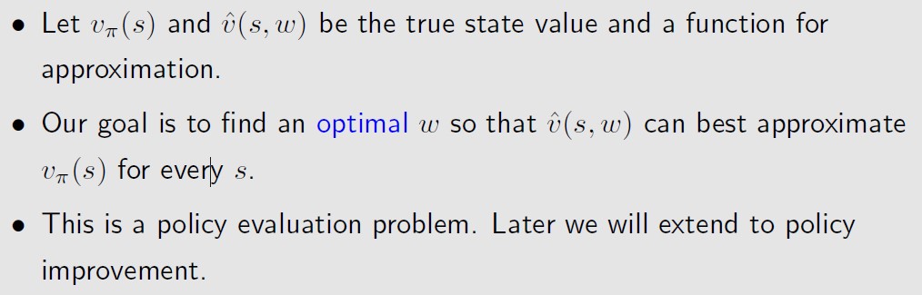
需要2个步骤，

1. The first step is to define an objective function.
2. The second step is to derive algorithms optimizing the objective function.

 

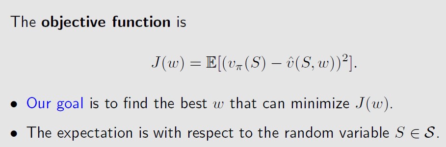
objective function如上图所示，是个期望的形式，因为S是个随机变量，即agent所处的状态s是

个随机变量。

S的概率分布有很多形式，比如均匀分布，

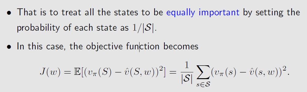
均匀分布的情况下，J（w)就是求平均值（期望的本质 就是求和）

但是this way does not consider the real dynamics of the Markov process under the given policy.

 

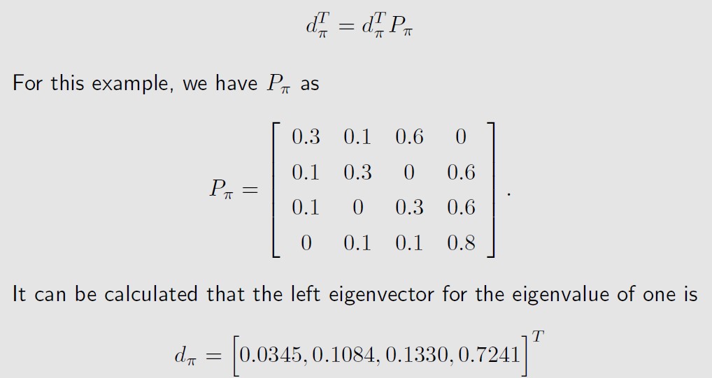
第二种分布是stationary distribution

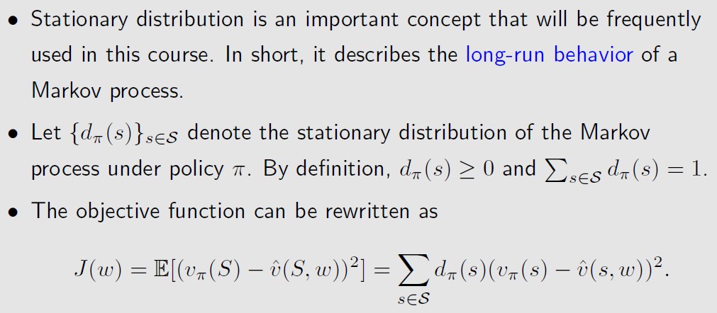
Since more frequently visited states have higher values of dπ(s), their

weights in the objective function are also higher than those rarely

visited states. 也就是给定Policy π，按照这个策略进行trajectory的采样，那么dπ(s)就表示

访问到状态s的频率（概率 ），频率越高的状态，权重越高。

after the agent runs a long time following a policy, the probability that the agent is at any state can be described by this distribution.

 

假设现在的策略如下图左面所示，

 

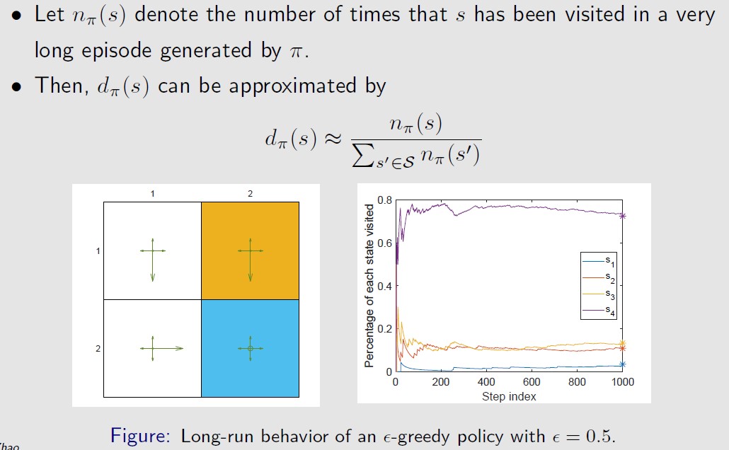
从右图中可以看出，随着step的增多，dπ(s)会逐渐收敛。

 

如果我们知道状态转移矩阵，就可以直接求出dπ(s)，dπ(s)是Pπ的特征向量。

 

有了objective function之后 ，就可以用梯度下降的方法来求w，

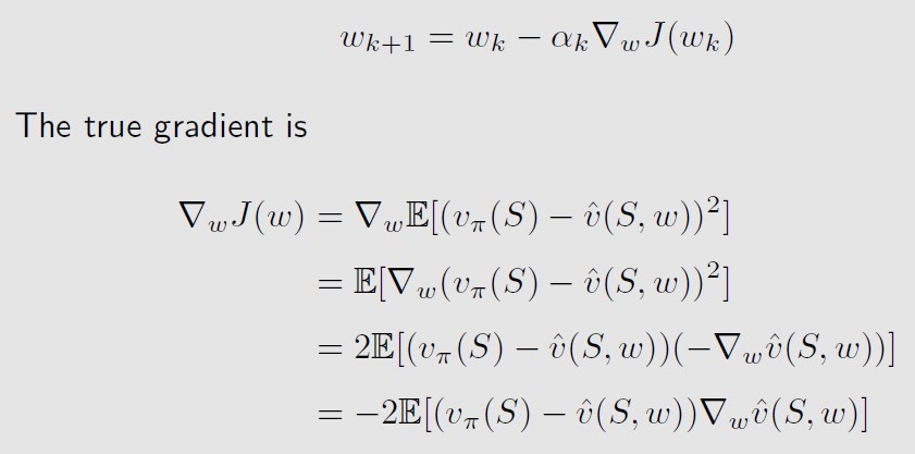
The true gradient above involves the calculation of an expectation.

上式左边是真实梯度，也是个期望的形式，We can use the stochastic gradient to replace the true gradient，我们可以用随机梯度来作为期望的估计，代替期望值（代替真实梯度）

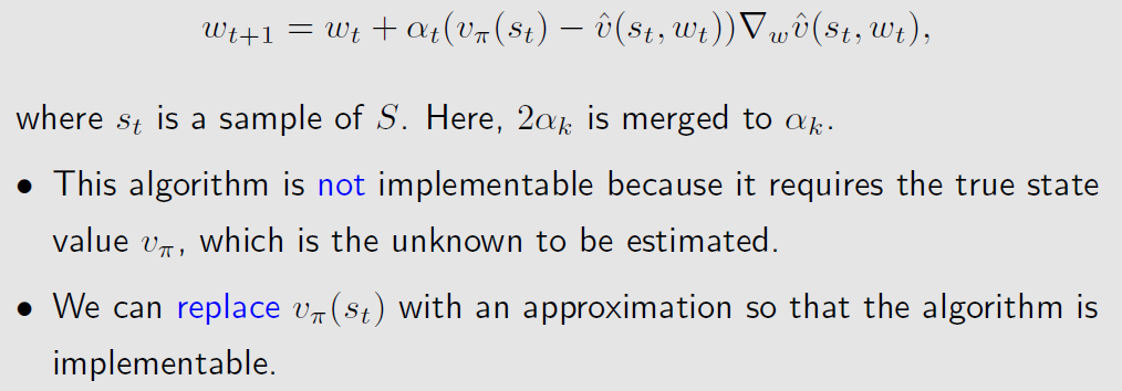
上式这个算法要求我们知道真实的state value vπ（s)，但是我们不知道vπ（s)，我们可以用一个估计值

来代替vπ（s)，可以用之前学过的monte carlo和TD算法来估计，

 

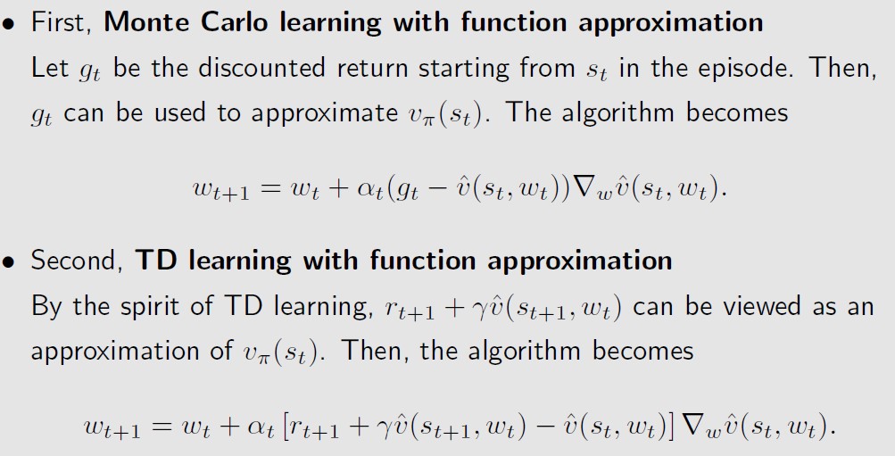
以TD算法为例，伪代码如下

 

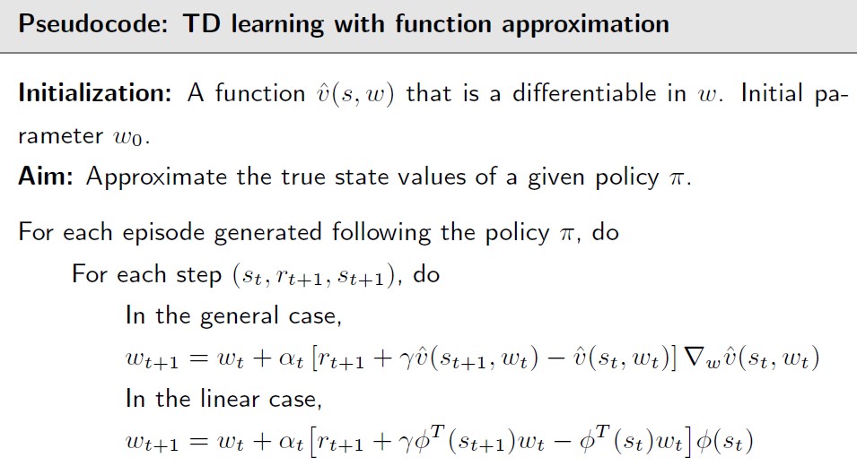
关于的具体形式，比如是w的线性函数，此时w是个向量[w1,w2,w3,…]，Ф可以是多

项式基，也可以是傅里叶基数

 

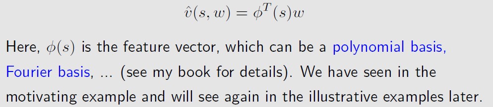
也可以是个神经网络，

The input of the NN is the state, the output is  and the network parameter is w.

 

Disadvantages of linear function approximation:

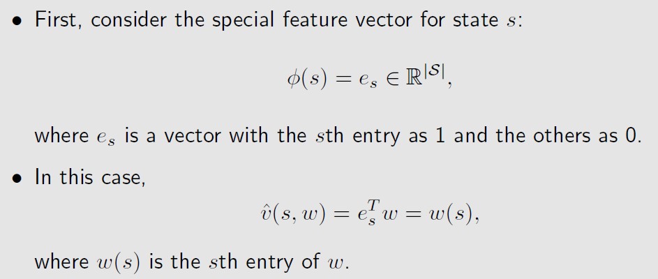
• Difficult to select appropriate feature vectors.

Advantages of linear function approximation:

• The theoretical properties of the TD algorithm in the linear case can be much better understood than in the nonlinear case.
• Linear function approximation is still powerful in the sense that the tabular representation is merely a special case of linear function approximation.

 

表格形式可以看成是 的线性形式的一种特殊情况，即状态s对应位置上的值是1，其实是0