CS336-2025-lec2

2025年8月8日

20:04

PyTorch, resource accounting

 

1.

Question: How long would it take to train a 70B parameter model on 15T tokens on 1024 H100s?

total_flops = 6 * 70e9 * 15e12 # @inspect total_flops #这里为什么是6，因为前向传播的计算量是2倍参数量*token数量，反向传播的计算量是4倍的参数量*token数量。

assert h100_flop_per_sec == 1979e12 / 2

mfu = 0.5

flops_per_day = h100_flop_per_sec * mfu * 1024 * 60 * 60 * 24 # @inspect flops_per_day

days = total_flops / flops_per_day # @inspect days

 

 

Question: What's the largest model that can you can train on 8 H100s using AdamW (naively)?

h100_bytes = 80e9 # @inspect h100_bytes

bytes_per_parameter = 4 + 4 + (4 + 4) # parameters, gradients, optimizer state @inspect bytes_per_parameter

num_parameters = (h100_bytes * 8) / bytes_per_parameter # @inspect num_parameters

Caveat 1: we are naively using float32 for parameters and gradients. We could also use bf16 for parameters and gradients (2 + 2) and keep an extra float32 copy of the parameters (4). This doesn't save memory, but is faster.  

[Rajbhandari+ 2019]

Caveat 2: activations are not accounted for (depends on batch size and sequence length).

 

 

One matrix in the feedforward layer of GPT-3:

assert get_memory_usage(torch.empty(12288 * 4, 12288)) == 2304 * 1024 * 1024  # 2.3 GB 一个全连接层就是2.3G

 

 



 



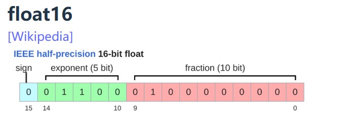
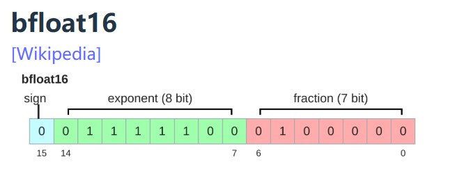
Google Brain developed bfloat (brain floating point) in 2018 to address this issue.

 bfloat16 uses the same memory as float16 but has the same dynamic range as float32!

 The only catch is that the resolution is worse, but this matters less for deep learning.

 

Implications on training:

• Training with float32 works, but requires lots of memory.
• Training with fp8, float16 and even bfloat16 is risky, and you can get instability.(用低精度的数据类型进行训练，可能会不稳定，数值上溢或下溢)
• Solution (later): use mixed precision training, see mixed_precision_training 解决方法是混合精度训练

 

2.Tensor

 What are tensors in PyTorch?

    PyTorch tensors are pointers into allocated memory

    ...with metadata describing how to get to any element of the tensor. 元信息就是stride，每个维度的步长



 

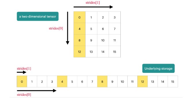
To go to the next row (dim 0), skip 4 elements in storage.

assert x.stride(0) == 4

 

To go to the next column (dim 1), skip 1 element in storage.

assert x.stride(1) == 1

 

To find an element:

r, c = 1, 2

index = r * x.stride(0) + c * x.stride(1) # @inspect index

assert index == 6

 

 

Many operations simply provide a different view of the tensor.

This does not make a copy, and therefore mutations in one tensor affects the other.大多数tensor的操作都不是复制操作，而是返回了tensor的视图，意味着一个变了，另一个也会变。

 

Get row 0:

y = x[0] # @inspect y

assert torch.equal(y, torch.tensor([1., 2, 3]))

assert same_storage(x, y)

 

Get column 1:

y = x[:, 1] # @inspect y

assert torch.equal(y, torch.tensor([2, 5]))

assert same_storage(x, y)

 

View 2x3 matrix as 3x2 matrix:

y = x.view(3, 2) # @inspect y

assert torch.equal(y, torch.tensor([[1, 2], [3, 4], [5, 6]]))

assert same_storage(x, y)

 

Transpose the matrix:

y = x.transpose(1, 0) # @inspect y

assert torch.equal(y, torch.tensor([[1, 4], [2, 5], [3, 6]]))

assert same_storage(x, y)

 

Check that mutating x also mutates y.

x[0][0] = 100 # @inspect x, @inspect y

assert y[0][0] == 100

 

Note that some views are non-contiguous entries, which means that further views aren't possible. (view只能对连续张量使用，什么是连续张量，就是数据在内存中的存储位置是连续的，不是跳跃的，如果对tensor进行遍历，只需要按顺序连续访问内存空间即可。reshape不要求tensor连续。)

x = torch.tensor([[1., 2, 3], [4, 5, 6]]) # @inspect x

y = x.transpose(1, 0) # @inspect y

assert not y.is_contiguous()

try:

y.view(2, 3)

assert False

except RuntimeError as e:

assert "view size is not compatible with input tensor's size and stride" in str(e)

 

One can enforce a tensor to be contiguous first:

y = x.transpose(1, 0).contiguous().view(2, 3) # @inspect y

assert not same_storage(x, y)

 

Views are free, copying take both (additional) memory and compute.

 

 

 

Einsum is generalized matrix multiplication with good bookkeeping.爱因斯坦求和主要是方便阅读

Define two tensors:

x: Float[torch.Tensor, "batch seq1 hidden"] = torch.ones(2, 3, 4) # @inspect x

y: Float[torch.Tensor, "batch seq2 hidden"] = torch.ones(2, 3, 4) # @inspect y

 

Old way:

z = x @ y.transpose(-2, -1) # batch, sequence, sequence @inspect z

 

New (einops) way:

z = einsum(x, y, "batch seq1 hidden, batch seq2 hidden -> batch seq1 seq2") # @inspect z

 

Dimensions that are not named in the output are summed over.

>

 

3. Computational cost

3.1 前向传播的计算量

    A floating-point operation (FLOP) is a basic operation like addition (x + y) or multiplication (x y).加法或乘法算一次FLOP。

 

As motivation, suppose you have a linear model.

• We have n points
• Each point is d-dimsional
• The linear model maps each d-dimensional vector to a k outputs

 

B = 1024

D = 256

K = 64

 

device = get_device()

x = torch.ones(B, D, device=device)

w = torch.randn(D, K, device=device)

y = x @ w

 

We have one multiplication (x[i][j] * w[j][k]) and one addition per (i, j, k) triple.

actual_num_flops = 2 * B * D * K  #全连接层的前向计算就是两个矩阵（B, D）和（D,K）做乘法，而矩阵乘法的计算量是 2 * B * D * K（新矩阵的每个元素都经过D次相乘和D-1次相加得到，共有B*K个元素）

 

 

In general, no other operation that you'd encounter in deep learning is as expensive as matrix multiplication for large enough matrices.通常来说，矩阵相乘的计算量是最大的。

 

Interpretation:

• B is the number of data points
• (D K) is the number of parameters
• FLOPs for forward pass is 2 (# tokens) (# parameters) #前向传播的计算量基本上可以认为是2*token数量*模型参数量。

It turns out this generalizes to Transformers (to a first-order approximation).

 

3.2 反向传播的计算量

 

#前向传播时，计算loss

Forward pass: compute loss

x = torch.tensor([1., 2, 3])

w = torch.tensor([1., 1, 1], requires_grad=True) # Want gradient

pred_y = x @ w

loss = 0.5 * (pred_y - 5).pow(2)

 

#反向传播时，计算梯度

Backward pass: compute gradients

loss.backward()

assert loss.grad is None

assert pred_y.grad is None

assert x.grad is None

assert torch.equal(w.grad, torch.tensor([1, 2, 3]))

 

假设我们的model是这样的：

Model: x --w1--> h1 --w2--> h2 -> loss

x = torch.ones(B, D, device=device)

w1 = torch.randn(D, D, device=device, requires_grad=True)

w2 = torch.randn(D, K, device=device, requires_grad=True)

 

h1 = x @ w1

h2 = h1 @ w2

loss = h2.pow(2).mean()

 

• h1.grad = d loss / d h1
• h2.grad = d loss / d h2
• w1.grad = d loss / d w1
• w2.grad = d loss / d w2

 

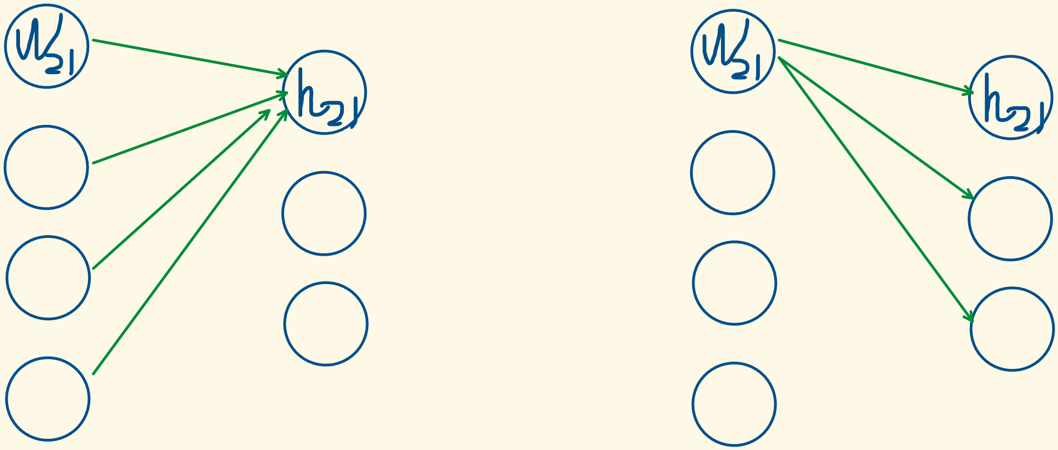
以计算w2矩阵的梯度为例，也就是计算w2对loss的影响力，假设已经有了h2.grad，也就是h2对loss的影响力，那么w2矩阵中某个元素对loss的影响力=w2矩阵中这个元素对h2矩阵中某一列中所有元素的影响力*h2矩阵中这一列的元素对loss的影响力，然后求和。计算量和矩阵乘法计算量一样。

 

h2 = h1 @ w2

（w2矩阵中每个元素对h2的梯度，也就是w2中每个元素对h2的影响力：w2中每个元素都影响h2的B个元素，也就是一列，所以w2中某个元素对h2的影响力=该元素对h2的B个元素的影响力求和）。

w2.grad = d loss / d w2 = (d h2 / d w2 )*(d loss/ d h2 )

 w2.grad[j,k] = sum_i h1[i,j] * h2.grad[i,k]

 

关于反向传播时w2梯度的计算量为什么和前向传播时矩阵相乘的计算量相等的画图解释：在前向传播时，h2的每个元素都是由前面4个节点求和得到的，同理，w2的每个元素都影响了后面的3个节点，也就是，w2每个元素的梯度也是要由后面3个节点求和得到，因此，反向传播和前向传播的计算量是相同的。

但是，我们不仅需要计算w2的梯度，还需要计算h1的梯度，h1的梯度是用于计算w1的梯度时用的，因为我们在计算w2梯度时，假设我们已经知道h2的梯度了。

也就是说，参数W和激活值h需要区分开，激活值 是输入值 x和输出y之间的中间产物，在反向传播时不仅需要计算参数W的梯度，还需要计算激活值的梯度。

 

 

Putting it togther:

• Forward pass: 2 (# data points) (# parameters) FLOPs
• Backward pass: 4 (# data points) (# parameters) FLOPs  # 参数w和激活值的梯度都需要计算
• Total: 6 (# data points) (# parameters) FLOPs

 

4. 其他

 

Randomness shows up in many places: parameter initialization, dropout, data ordering, etc.

For reproducibility, we recommend you always pass in a different random seed for each use of randomness.

Determinism is particularly useful when debugging, so you can hunt down the bug.

 

There are three places to set the random seed which you should do all at once just to be safe.

#有3处常见的随机性

# Torch

seed = 0

torch.manual_seed(seed)

 

# NumPy

import numpy as np

np.random.seed(seed)

 

# Python

import random

random.seed(seed)

 

#输入数据很大时 (LLaMA data is 2.8TB).，可以惰性加载，一次只从硬盘中读取一部分数据，而不是将数据一次性加载到内存中

You can load them back as numpy arrays.

Don't want to load the entire data into memory at once (LLaMA data is 2.8TB).

Use memmap to lazily load only the accessed parts into memory.

data = np.memmap("data.npy", dtype=np.int32)

 

训练过程中保存时，不仅需要保存模型，还需要保存optimizer

#optimizer中保存了参数的历史梯度信息，如

• momentum = SGD + exponential averaging of grad
• AdaGrad = SGD + averaging by grad^2
• RMSProp = AdaGrad + exponentially averaging of grad^2
• Adam = RMSProp + momentum

 

Save the checkpoint:

checkpoint = {

"model": model.state_dict(),

"optimizer": optimizer.state_dict(),

}

torch.save(checkpoint, "model_checkpoint.pt")

 

数据类型的选择：

 

Choice of data type (float32, bfloat16, fp8) have tradeoffs.

• Higher precision: more accurate/stable, more memory, more compute
• Lower precision: less accurate/stable, less memory, less compute

 

How can we get the best of both worlds?

Solution: use float32 by default, but use {bfloat16, fp8} when possible.

 

A concrete plan:

• #激活值用bf16，参数值和梯度用fl32，
• Use {bfloat16, fp8} for the forward pass (activations).
• Use float32 for the rest (parameters, gradients).

 

• Mixed precision training

 

[Micikevicius+ 2017]

 

 

Pytorch has an automatic mixed precision (AMP) library.

 

https://pytorch.org/docs/stable/amp.html

https://docs.nvidia.com/deeplearning/performance/mixed-precision-training/

 

 

NVIDIA's Transformer Engine supports FP8 for linear layers

Use FP8 pervasively throughout training  

[Peng+ 2023]