GNN
2025年9月21日
9:14
A Gentle Introduction to Graph Neural Networks来自 <https://distill.pub/2021/gnn-intro/>
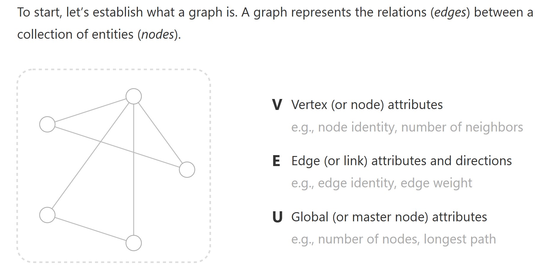
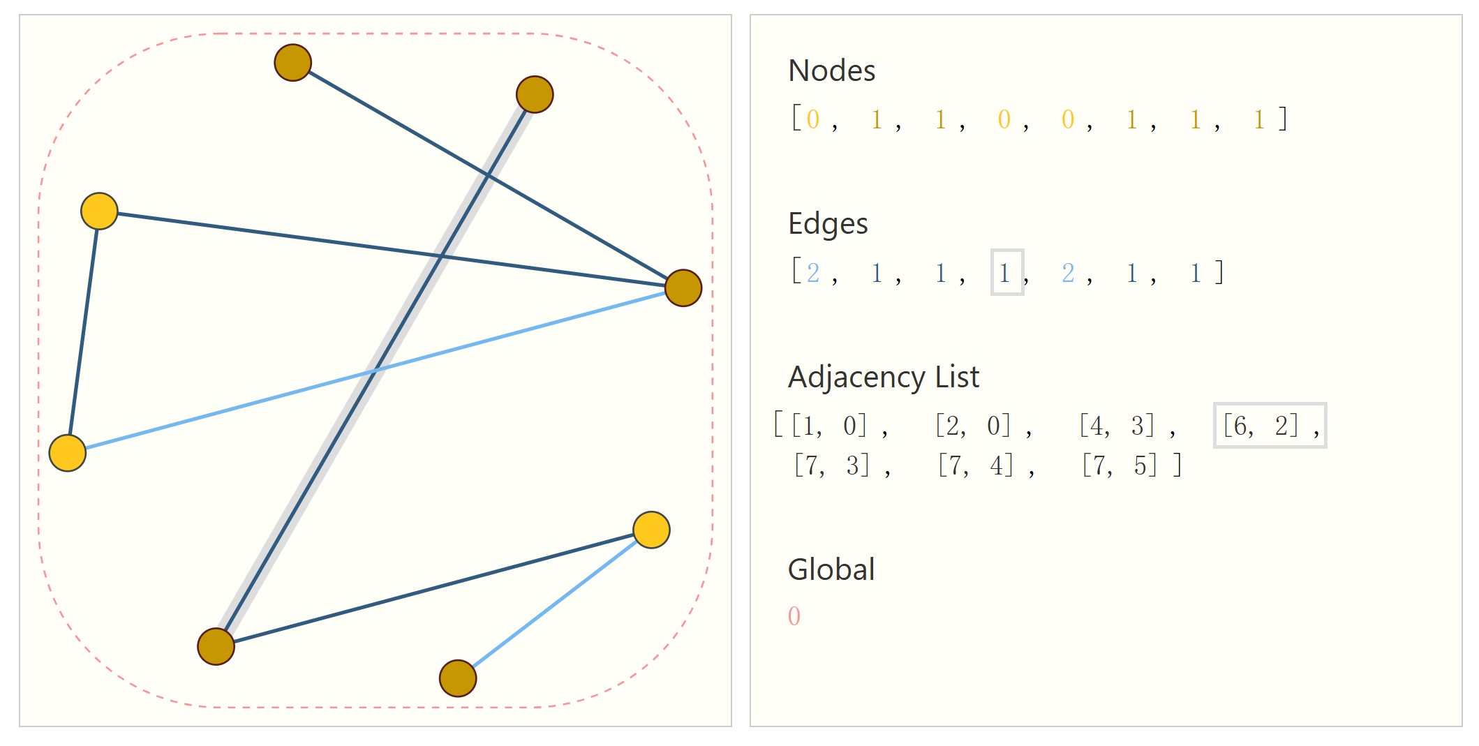
图由节点V,边E,全局信息U组成。
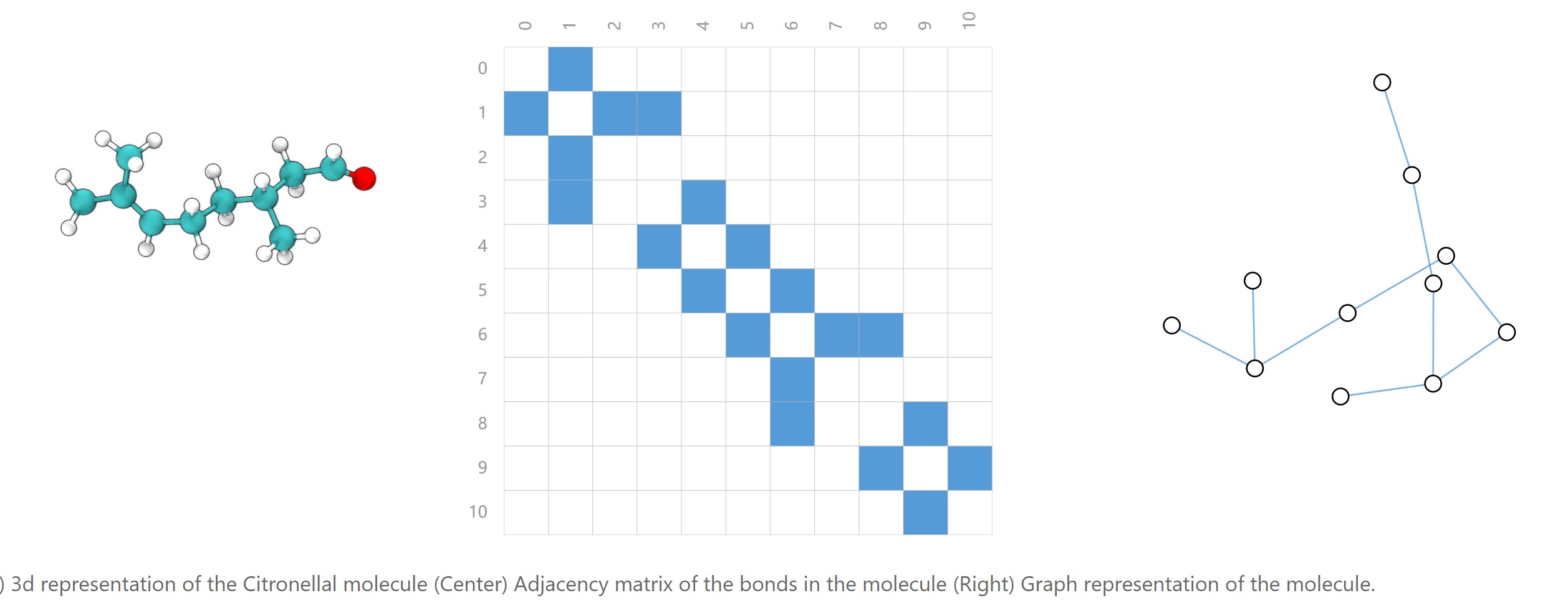
可以用邻接矩阵表示图的连通性,即边,如下图中间的矩阵,对于无向图来说,邻接矩阵是对称的。
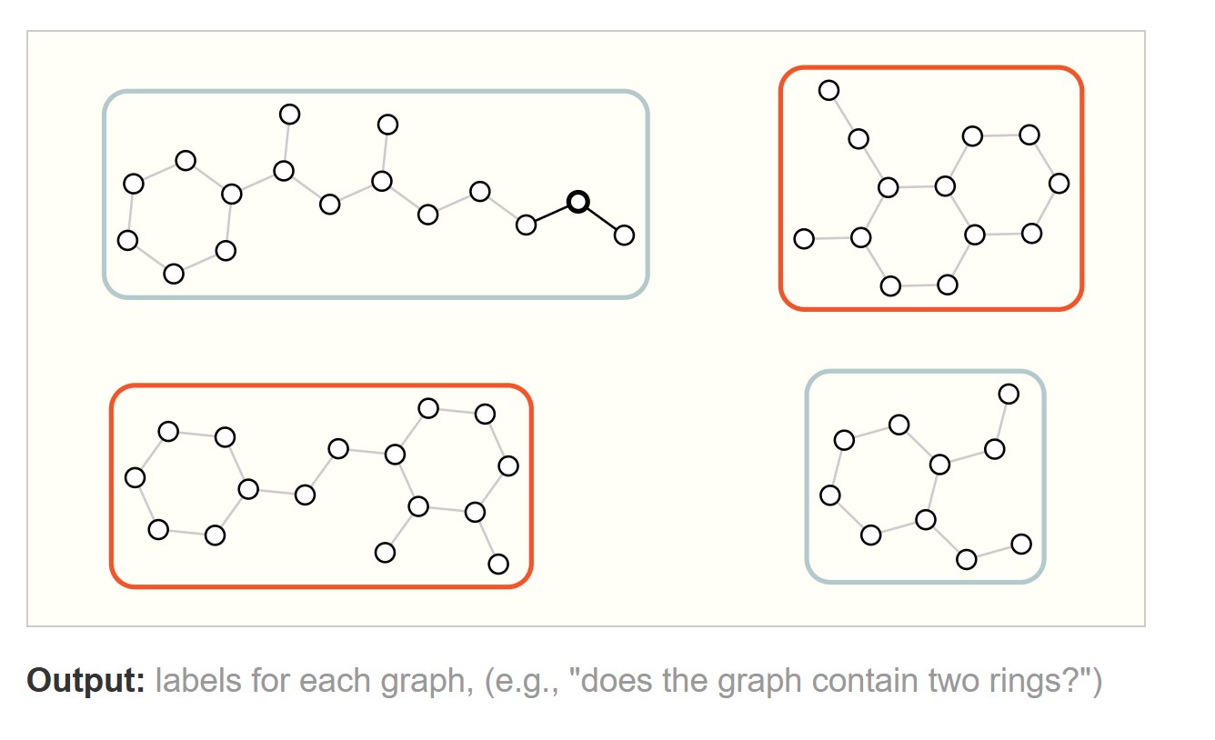
There are three general types of prediction tasks on graphs: graph-level, node-level, and edge-level.
- Graph-level task
- Node-level task
预测每个节点的性质
- Edge-level task
预测每条边的性质
The challenges of using graphs in machine learning
1.图的连通性表示。可以用邻接矩阵表示,但是对于一张大图来说,邻接矩阵通常是稀疏的,稀疏矩阵的处理效率较低。并且,同一张图可以有多个邻接矩阵的表示(只需要变换节点的顺序,但还是同一张graph,如下图所示,这些矩阵表示都是同一张graph),也就是说graph是permutation invariant,邻接矩阵变了,图是不变的,但是我们的神经网络的输出通常是变的。
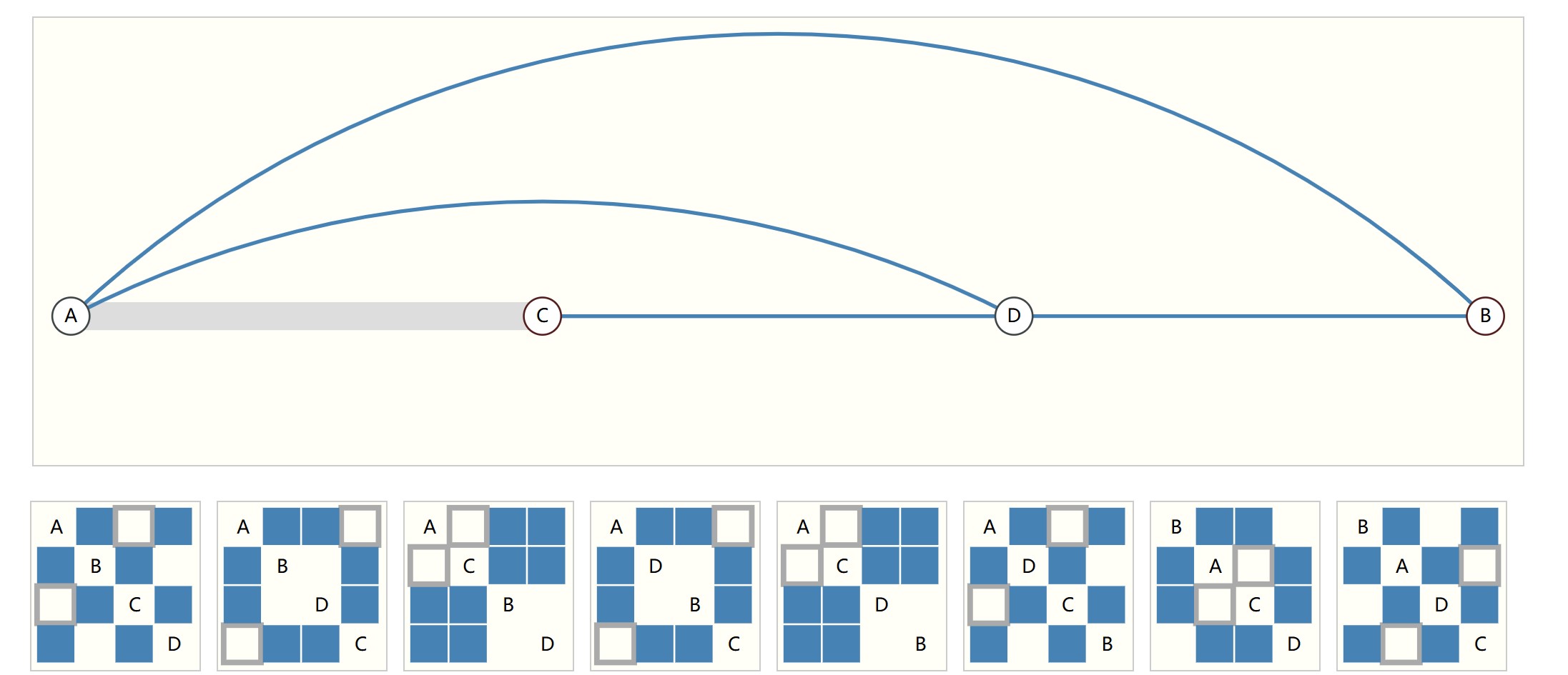
解决方法是用邻接列表来代替邻接矩阵,只存储边。
Graph Neural Networks
A GNN is an optimizable transformation on all attributes of the graph (nodes, edges, global-context) that preserves graph symmetries (permutation invariances).
GNN就是一种作用在图的节点、边、全局信息上的一种可优化的变换,同时不改变图的结构。
GNNs adopt a “graph-in, graph-out” architecture meaning that these model types accept a graph as input, with information loaded into its nodes, edges and global-context, and progressively transform these embeddings, without changing the connectivity of the input graph.
GNN的输入是图,输出也是图。
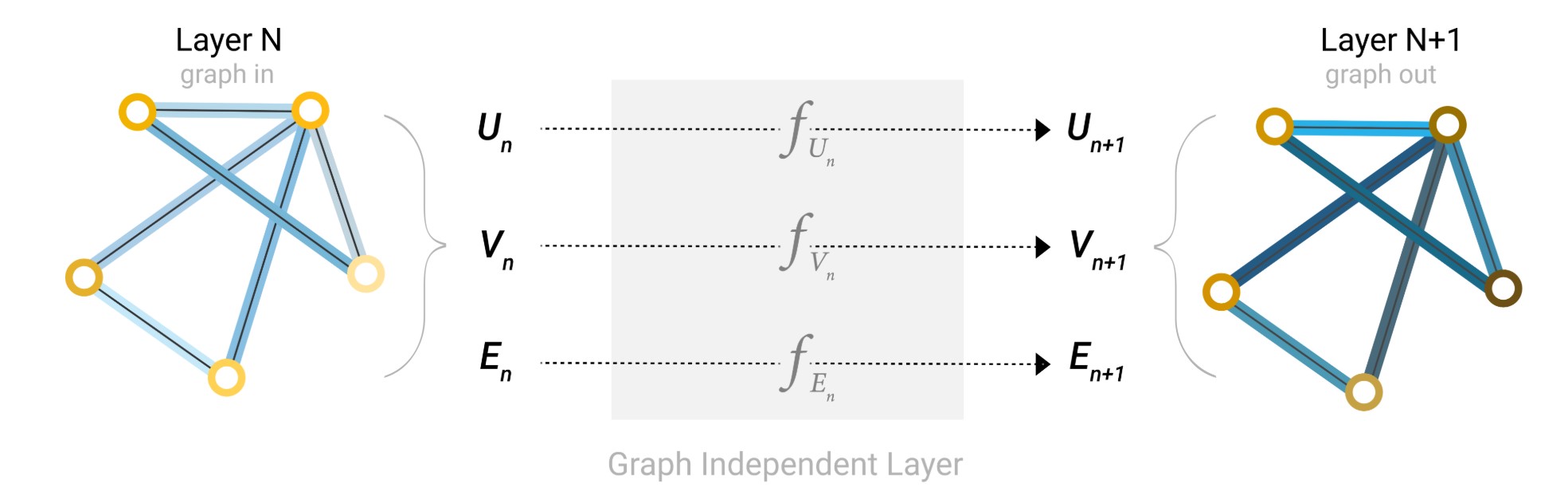
- 最简单的GNN架构:对V、E、U分别单独处理,不考虑连通性。
We will start with the simplest GNN architecture, one where we learn new embeddings for all graph attributes (nodes, edges, global), but where we do not yet use the connectivity of the graph.
For simplicity, the previous diagrams used scalars to represent graph attributes; in practice feature vectors, or embeddings, are much more useful.
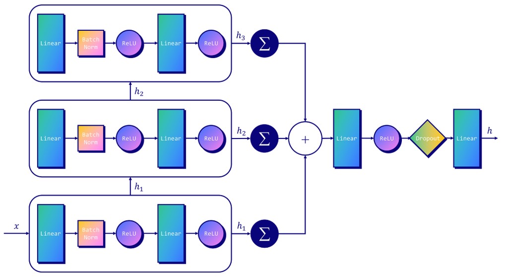
This GNN uses a separate multilayer perceptron (MLP) (or your favorite differentiable model) on each component of a graph; we call this a GNN layer. For each node vector, we apply the MLP and get back a learned node-vector. We do the same for each edge, learning a per-edge embedding, and also for the global-context vector, learning a single embedding for the entire graph.
We only use connectivity when pooling information for prediction. 在预测时,假设我们缺失某个节点或边的属性,我们可以利用连通性,汇聚邻居节点或边的信息。
- GCN
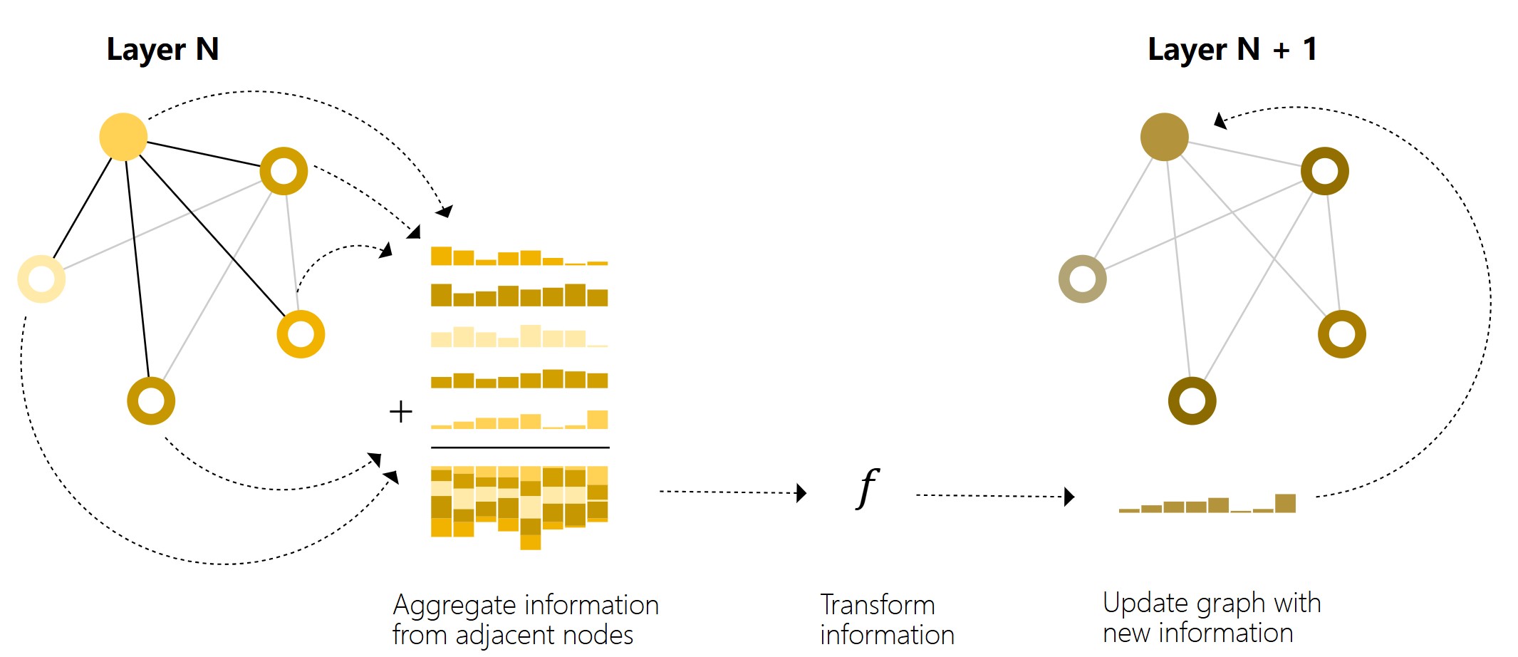
Message passing。
利用连通性,在每一层,对一个节点,汇聚其周围邻居信息之后 ,然后再进入MLP。
Message passing works in three steps:
- For each node in the graph, gather all the neighboring node embeddings (or messages), which is the g function described above.
- Aggregate all messages via an aggregate function (like sum).
- All pooled messages are passed through an update function, usually a learned neural network.
This is reminiscent of standard convolution: in essence, message passing and convolution are operations to aggregate and process the information of an element’s neighbors in order to update the element’s value. In graphs, the element is a node, and in images, the element is a pixel. However, the number of neighboring nodes in a graph can be variable, unlike in an image where each pixel has a set number of neighboring elements.还有一点和图像中的卷积不一样,就是图像中的卷积核中定义了不同位置的权重 ,而这里所有邻居的权重都是1,直接相加,而图像中的卷积相当于是加权和。
上图表示的是Schematic for a GCN architecture, which updates node representations of a graph by pooling neighboring nodes at a distance of one degree。
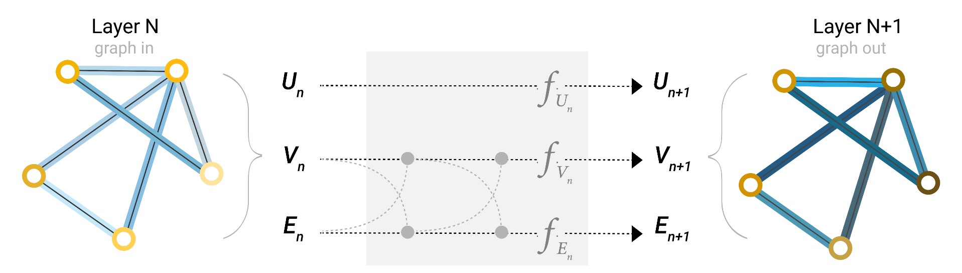
除了将周围节点的信息汇聚到节点外,还可以将周围边的信息汇聚到某个节点,以及将某个边连接的两个节点的信息汇聚到这条边上,如果节点和边的embedding不一样的话,进行一个线性变换(投影)即可。完成了信息传递之后,再输入到各自的MLP即可。如下图所示,可以先将节点信息汇聚到边,然后再将更新后的边的信息汇聚到点,也可以反过来,具体按照哪个顺序,不确定,可以同时更新。
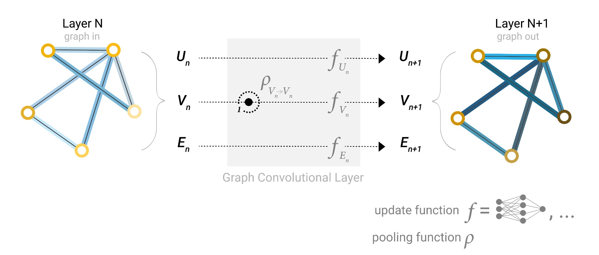
还可以在message passing中加上全局信息U,架构如下图所示
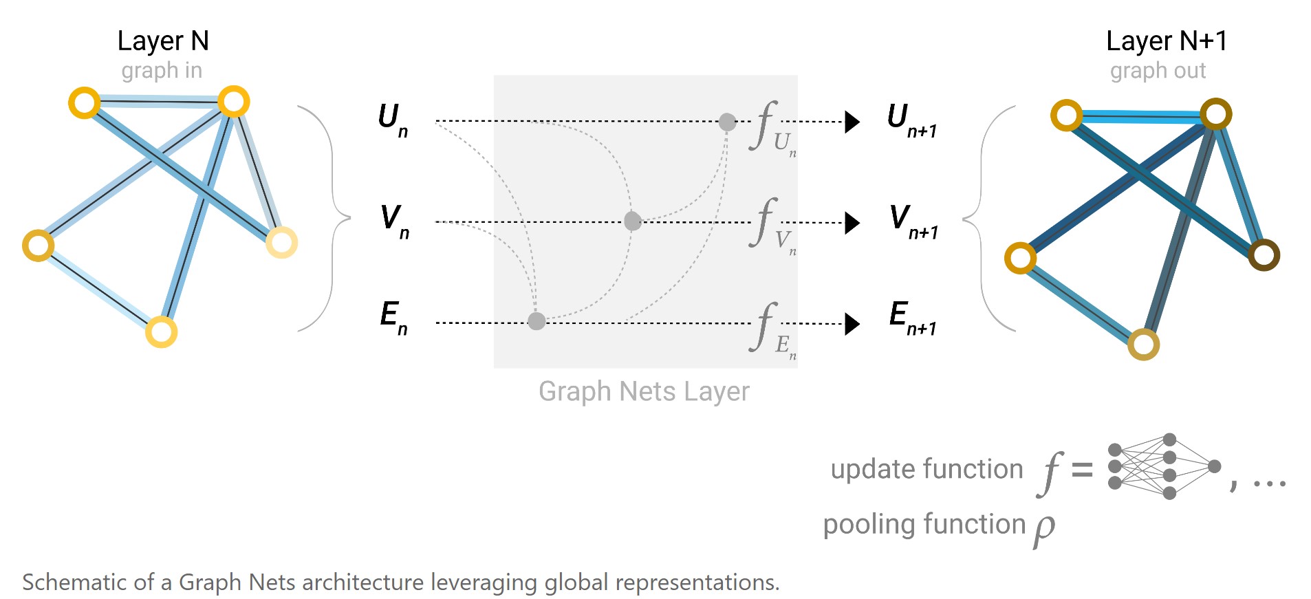
In this view all graph attributes have learned representations, so we can leverage them during pooling by conditioning the information of our attribute of interest with respect to the rest. For example, for one node we can consider information from neighboring nodes, connected edges and the global information. To condition the new node embedding on all these possible sources of information, we can simply concatenate them. Additionally we may also map them to the same space via a linear map and add them or apply a feature-wise modulation layer, which can be considered a type of featurize-wise attention mechanism.
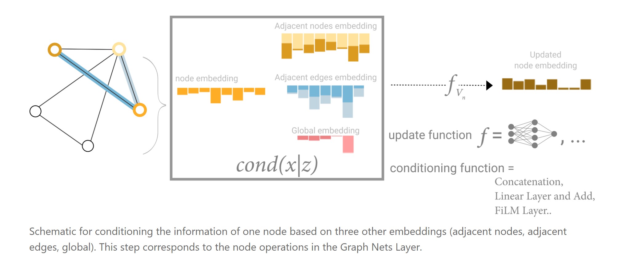
如下图所示,对每一层来说,以某个节点的embedding更新为例,除了用自己的embedding和邻居节点的embedding外,还用了所有相连的边的embedding以及全局信息embedding,cond(x|z)表示可以对这4个信息进行concat,也可以投影后相加,也可以做film,特征层面上的attention。然后再经过f_Vn(MLP),得到新的节点的embedding。
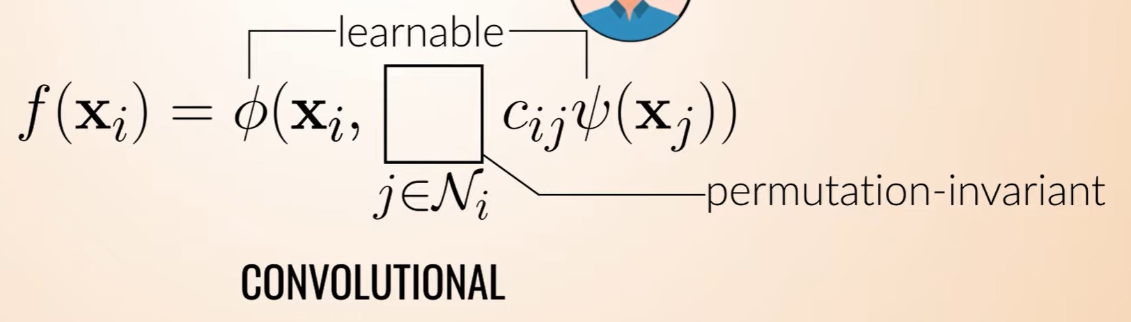
这个图是先对邻居节点xj进行变换,然后每个xj都有一个权重 ,如果这些权重是固定不变的,就类似于卷积核中的参数,也就是说邻居节点的权重取决于邻居的位置?
所以是先对xj变换,再汇聚,还是先汇聚,再对汇聚后的向量做变换?都可以?对简单的求和汇聚的GCN来说,没有区别,Wx1+Wx2+Wx3=W(x1+x2+x3)
GCN:
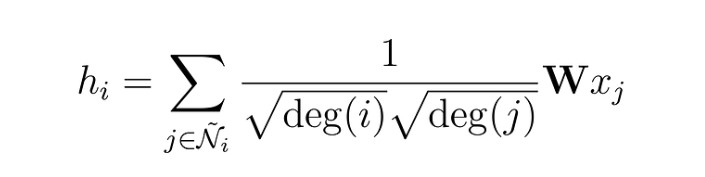
W*x_j 是对每个邻居节点的embedding做linear layer线性变换,所有的节点共享一个W。This operation is called convolution, or neighborhood aggregation,邻居汇聚也称为卷积。
GAT:https://mlabonne.github.io/blog/posts/2022-03-09-Graph_Attention_Network.html
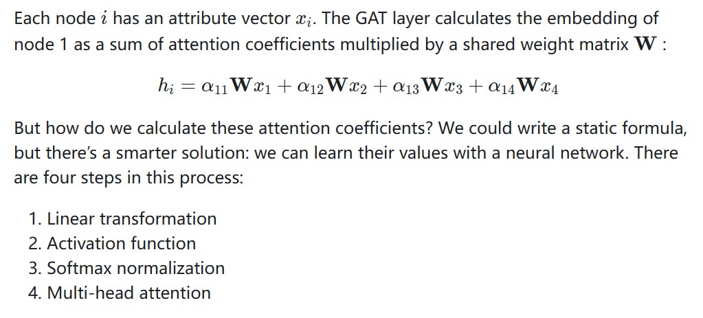
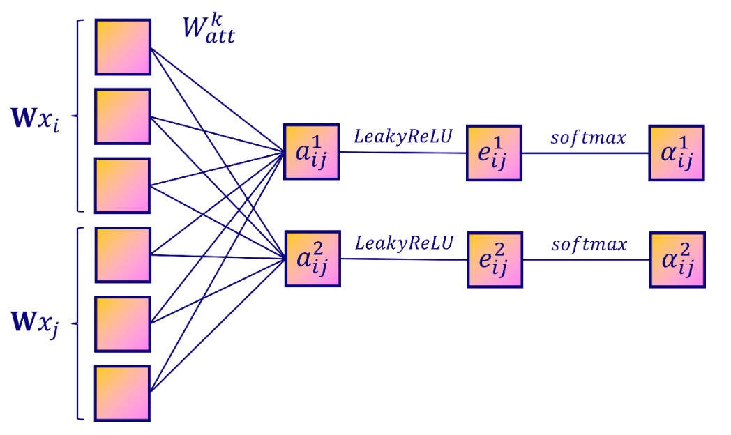
1. Linear transformation
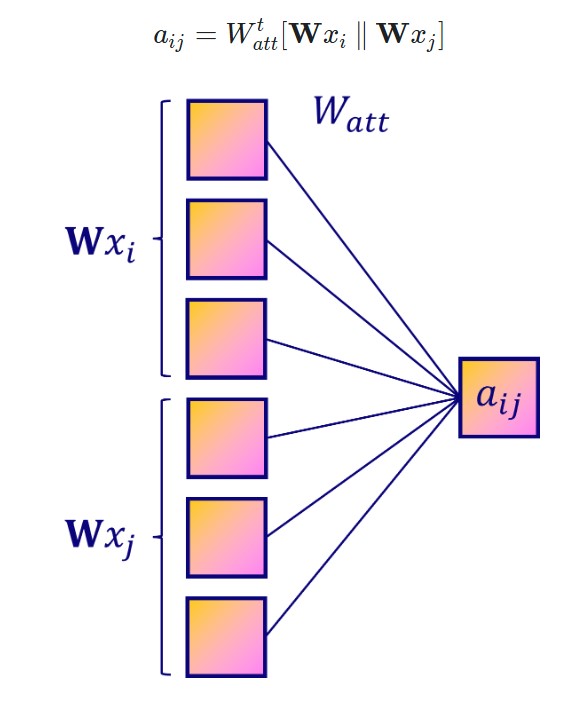
To calculate the attention coefficient, we need to consider pairs of nodes. An easy way to create these pairs is to concatenate attribute vectors from both nodes.
Then, we can apply a new linear transformation with a weight matrix W_att:
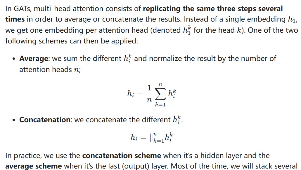
4. Multi head attention
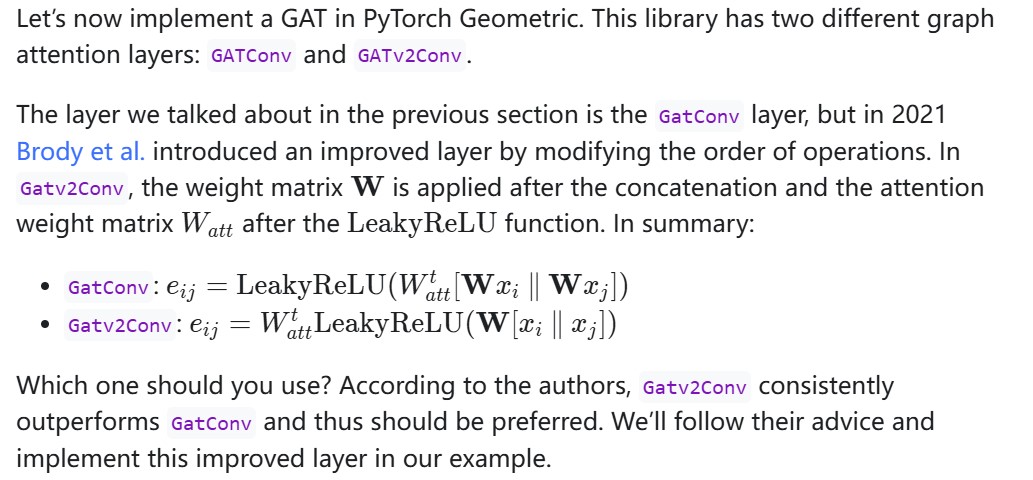
在pyG中,有两种GAT layer
import torch.nn.functional as F
from torch.nn import Linear, Dropout
from torch_geometric.nn import GCNConv, GATv2Conv
class GCN(torch.nn.Module):
    """Graph
Convolutional Network"""
    def __init__(self, dim_in,
dim_h, dim_out):
super().__init__()
      self.gcn1 = GCNConv(dim_in,
dim_h)
      self.gcn2 = GCNConv(dim_h,
dim_out)
      self.optimizer =
torch.optim.Adam(self.parameters(),
lr=0.01,
weight_decay=5e-4)
    def forward(self, x,
edge_index):
        h = F.dropout(x, p=0.5,
training=self.training)
        h = self.gcn1(h,
edge_index).relu()
        h = F.dropout(h, p=0.5,
training=self.training)
        h = self.gcn2(h,
edge_index)
        return h,
F.log_softmax(h, dim=1)
class GAT(torch.nn.Module):
    """Graph
Attention Network"""
    def __init__(self, dim_in,
dim_h, dim_out, heads=8):
super().__init__()
        self.gat1 =
GATv2Conv(dim_in, dim_h, heads=heads)
        self.gat2 =
GATv2Conv(dim_h*heads, dim_out, heads=1)
        self.optimizer =
torch.optim.Adam(self.parameters(),
lr=0.005,
weight_decay=5e-4)
    def forward(self, x,
edge_index):
        h = F.dropout(x, p=0.6,
training=self.training)
        h = self.gat1(h,
edge_index)
h = F.elu(h)
        h = F.dropout(h, p=0.6,
training=self.training)
        h = self.gat2(h,
edge_index)
        return h,
F.log_softmax(h, dim=1)
def accuracy(pred_y, y):
    """Calculate
accuracy."""
    return ((pred_y == y).sum() /
len(y)).item()
def train(model, data):
    """Train a GNN
model and return the trained model."""
    criterion =
torch.nn.CrossEntropyLoss()
optimizer = model.optimizer
epochs = 200
model.train()
for epoch in range(epochs+1):
# Training
optimizer.zero_grad()
        _, out = model(data.x,
data.edge_index)
        loss =
criterion(out[data.train_mask], data.y[data.train_mask])
        acc =
accuracy(out[data.train_mask].argmax(dim=1), data.y[data.train_mask])
loss.backward()
optimizer.step()
# Validation
        val_loss =
criterion(out[data.val_mask], data.y[data.val_mask])
        val_acc =
accuracy(out[data.val_mask].argmax(dim=1), data.y[data.val_mask])
        # Print metrics every 10
epochs
if(epoch % 10 == 0):
            print(f'Epoch
{epoch:>3} | Train Loss: {loss:.3f} | Train Acc: '
f'{acc*100:>6.2f}% | Val Loss: {val_loss:.2f} | '
                  f'Val Acc:
{val_acc*100:.2f}%')
return model
@torch.no_grad()
def test(model, data):
    """Evaluate
the model on test set and print the accuracy score."""
model.eval()
    _, out = model(data.x,
data.edge_index)
    acc =
accuracy(out.argmax(dim=1)[data.test_mask], data.y[data.test_mask])
return acc
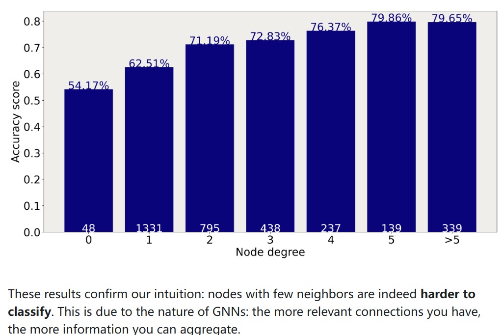
一个节点的邻居越多,分类准确率越高。
GraphSAGE
对batch中的所有target node进行采样,每个target
node采出一个子图来,然后合并为一张图,用来message
passing,而不是用整个完整的图进行message
passing。mini-batching is incredibly efficient,训练速度比GAT快多了。
GIN 图同构网络
核心目标是实现图同构识别(判断两个图是否结构相同),并在此基础上学习具有强区分性的图表示。它的设计直接对标图同构测试的经典算法(Weisfeiler-Lehman 算法),理论上能区分任何非同构的图,更适合图级任务(如图分类、分子属性预测)。GIN和GCN两者的核心差异体现在邻居信息的聚合方式上,这直接决定了它们对图结构的捕捉能力。
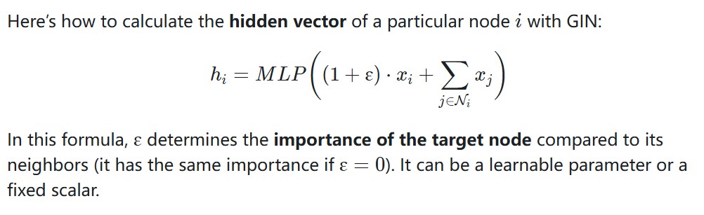
对所有节点的embedding进行汇聚,得到全图的embedding信息,具体做法:
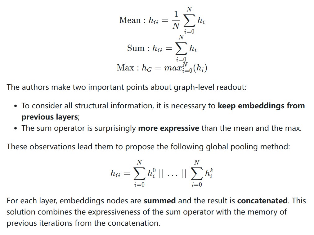
也就是在每一层的计算中,sum所有节点得到全图的embedding,然后把每一层的graph embedding concat起来。