量化-2
2025年9月26日
14:36
- Post-Training Quantization (PTQ) is a straightforward technique where the weights of an already trained model are converted to lower precision without necessitating any retraining. Although easy to implement, PTQ is associated with potential performance degradation .训练完后再量化
- Quantization-Aware Training (QAT) incorporates the weight conversion process during the pre-training or fine-tuning stage, resulting in enhanced model performance. However, QAT is computationally expensive and demands representative training data.
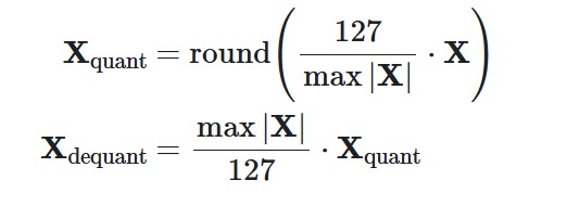
- With absmax quantization, the original number is divided by the absolute maximum value of the tensor and multiplied by a scaling factor (127) to map inputs into the range [-127, 127]. To retrieve the original FP16 values, the INT8 number is divided by the quantization factor, acknowledging some loss of precision due to rounding.
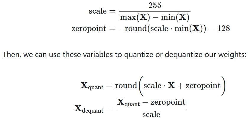
- With zero-point quantization, we can consider asymmetric input distributions, which is useful when you consider the output of a ReLU function (only positive values) for example. The input values are first scaled by the total range of values (255) divided by the difference between the maximum and minimum values. This distribution is then shifted by the zero-point to map it into the range [-128, 127] (notice the extra value compared to absmax). First, we calculate the scale factor and the zero-point value:
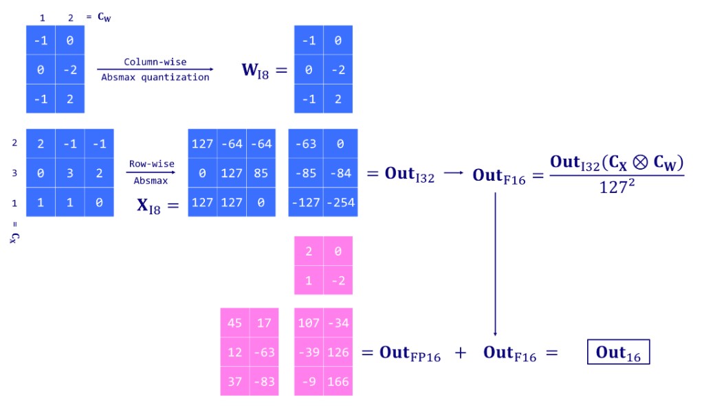
- Extract columns from the input hidden states containing outlier features using a custom threshold.
- Perform the matrix multiplication of the outliers using FP16 and the non-outliers using INT8 with vector-wise quantization (row-wise for the hidden state and column-wise for the weight matrix ).
- Dequantize the non-outlier results (INT8 to FP16) and add them to the outlier results to get the full result in FP16.
- 原始笨办法(OBQ):检查所有食材(权重),先找到那个用“勺”代替“克”后对菜品味道影响最小的食材进行替换。换完一个后,重新评估下一个对味道影响最小的... 这个过程非常耗时。
- GPTQ的洞察:对于一本超级厚的食谱(大模型),其实按固定的顺序(比如从第一列食材到最后一列)来处理,最终效果差不多。因为即使某个食材单独替换影响大,但当轮到它时,其他大部分食材已经调整完了,它的错误也就很难扩散了。
- 做法:GPTQ就简单地从左到右一列一列地处理食谱矩阵。这样做的好处是,对于同一列食材,可以集中做一次计算,然后应用到所有菜品(行)上,效率极高。
- GPTQ的妙招:“偷懒”地批量处理。它把食谱分成多个章节(Block),比如每次处理128列。
- 做法:
- 在一个章节内,它专心致志地调整这几列的食材单位,并记录下调整所产生的误差(比如,把“5克盐”改成“1勺盐”,实际上可能只有4.8克,产生了0.2克的误差)。
- 在当前章节内部,它会根据这个误差,预先微调本章节内尚未处理的其他食材的用量,来补偿这个误差。比如,盐少放了0.2克,那就在后面处理“酱油”时,酌情多放一点来弥补咸味。
- 只有当一个章节全部处理完后,GPTQ才进行一次“全局更新”,把本章节累积的误差补偿应用到整本食谱剩余未处理的章节的所有食材上。
- GPTQ的保障:它使用了一种在数学上非常稳定可靠的工具,叫做Cholesky分解,来进行核心的误差计算和更新。这就像是用高精度的天平和一个严谨的数学公式来计算如何补偿误差,而不是凭感觉。
- 做法:在开始处理前,先用Cholesky分解预处理一下食谱(Hessian矩阵的逆),并加入一点“阻尼”(dampening)防止计算溢出。这让整个减肥过程非常稳健,不会因为数值问题而失败。
- 准备:拿出美食家的完整精细食谱(FP16模型权重),请来营养师(Cholesky分解)制定科学计划。
- 分章:把食谱分成几个大章(分批处理,如每次128列)。
- 处理章节:对当前章节,从左到右一列一列地:
- 量化:将食材单位从“克”改为“勺”(quant(w))。
- 计算误差:看看这次替换导致了多大的口味偏差(w - quant(w))。
- 局部补偿:立即在本章节内,调整后面尚未处理的食材用量,来弥补这个误差(利用营养师给的公式)。
- 全局更新:当前章节处理完后,根据本章节的总误差,去调整整本食谱后面所有章节的食材用量。
- 循环:移动到下一个章节,重复步骤3-4,直到处理完整本食谱。
- GPTQ保护的是整个模型结构的稳定性
- AWQ保护的是对最终输出影响大的敏感权重
- GPTQ通常按矩阵列或块进行量化
- AWQ可以做到更细粒度的权重级保护
- AWQ首先准备一些代表性的样本数据(比如一段文本),让模型“思考”一下。
- 它观察在 processing 这些数据时,哪些权重通道(通常以输出通道为单位)被激活得最强烈。这就像观察美食家做他的招牌菜时,哪些调料他用的最多、最讲究。
- 对于这些被识别出的重要权重通道,AWQ会决定“特殊照顾”。它会给这些通道计算一个大于1的缩放因子(scale)。
- AWQ不会像GPTQ那样逐个调整权重。它的核心操作是一个简单的每通道缩放(per-channel scaling)。
- 对模型的每个权重矩阵,根据侦察结果,对每个输出通道的权重乘以一个特定的缩放因子(重要的放大一点,不重要的可能缩小一点)。
- 然后,对这个缩放后的权重矩阵进行标准的、简单的四舍五入量化(RTN)。
We distinguish two main families of weight quantization techniques in the literature:
1.ABS和zero-point量化
In this section, we will implement two quantization techniques: a symmetric one with absolute maximum (absmax) quantization and an asymmetric one with zero-point quantization. In both cases, the goal is to map an FP32 tensor (original weights) to an INT8 tensor (quantized weights).
absmax是只考虑绝对值的最大值,zero-point考虑最大值-最小值,int8只能表示256个数,也就是[-127,127]的范围,
import torch
def absmax_quantize(X):
# Calculate scale
    scale = 127 /
 torch.max(torch.abs(X))
# Quantize
    X_quant = (scale *
 X).round()
# Dequantize
X_dequant = X_quant / scale
    return
 X_quant.to(torch.int8), X_dequant
进行abs或zero-point量化时,可以对某一层的所有参数tensor统一计算max,min来统一量化(per-layer),也可以对所有层的参数统一量化,也可以对单独的参数tensor单独计算max,min。在实际中常常用的是vector-wise quantization ,不再将整个张量(tensor)视为一个整体进行量化,而是沿着张量的某个维度(通常是通道维度或输入维度)将其划分为多个向量,然后对每个向量独立进行量化。这样做的好处是能更精细地适应数据内部的分布差异。一个张量中不同行或不同列的数值分布可能差异很大,为每个向量单独计算量化参数(如缩放因子)可以更好地捕捉这种局部特征,从而减少量化误差。
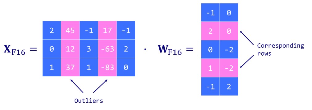
但是,However, even vector-wise quantization doesn’t solve the problem of outlier features. Outlier features are extreme values (negative or positive) that appear in all transformer layers when the model reach a certain scale (>6.7B parameters). This is an issue since a single outlier can reduce the precision for all other values. But discarding these outlier features is not an option since it would greatly degrade the model’s performance.
我们以一个简单的矩阵乘法为例,这是神经网络中最核心的运算之一: Y = X · W
其中:
X 是输入激活张量,形状为 [1, 4] (1个样本,4个特征)
W 是权重张量,形状为 [4, 3] (4个输入特征,3个输出特征)
Y 是输出张量,形状为 [1, 3]
假设我们的权重矩阵 W 如下:
输出通道 1 输出通道 2 输出通道 3
输入通道 1 1.2 0.8 -1.5
输入通道 2 2.1 -0.2 0.9
输入通道 3 -2.8 1.7 -0.1
输入通道 4 0.5 -1.1 2.0
方法一:Per-Tensor 量化(作为对比)
这是最粗的粒度。我们将整个 W 矩阵视为一个整体进行量化。
找出整个矩阵的绝对值最大值(absmax): absmax(W) = max(abs(-2.8), abs(2.1), ...) = 2.8
计算缩放因子(scale): 假设我们量化到 INT8(范围 [-127, 127]),则 scale = 127 / 2.8 ≈ 45.36
量化整个矩阵: W_quantized = round(W / scale)
问题: 我们可以看到,第3行第1列的值 -2.8 是一个“极端值”(在这个小例子中相当于 outlier)。因为它,缩放因子会变得很大(45.36),导致其他数值较小的值(如 0.8, -0.2)在量化后会失去大量精度,甚至被量化为0。
方法二:Vector-Wise 量化(按行量化)
这是更常见的做法。我们将 W 的每一行(对应一个输入通道,跨越所有输出通道)作为一个独立的向量进行量化。
按行找出绝对值最大值(absmax):
第 1 行 [1.2, 0.8, -1.5] -> absmax = 1.5
第 2 行 [2.1, -0.2, 0.9] -> absmax = 2.1
第 3 行 [-2.8, 1.7, -0.1] -> absmax = 2.8
第 4 行 [0.5, -1.1, 2.0] -> absmax = 2.0
为每一行计算独立的缩放因子(scale):
第 1 行 scale₁ = 127 / 1.5 ≈ 84.67
第 2 行 scale₂ = 127 / 2.1 ≈ 60.48
第 3 行 scale₃ = 127 / 2.8 ≈ 45.36
第 4 行 scale₄ = 127 / 2.0 = 63.5
按行量化矩阵:
量化第 1 行: round([1.2, 0.8, -1.5] / scale₁) ≈ round([0.014, 0.009, -0.018] * 84.67) ≈ [1, 1, -2]
量化第 2 行: round([2.1, -0.2, 0.9] / scale₂) ≈ round([0.035, -0.003, 0.015] * 60.48) ≈ [2, 0, 1]
... 以此类推。
优势: 现在,只有第3行受到了其内部极值 -2.8 的影响,缩放因子较小(45.36)。而其他行的数值因为有自己的缩放因子,得以更精确地表示。例如,第1行中的小值 0.8 现在可以被量化为 1,而不是像 per-tensor 量化中那样可能变成 0。
2.LLM.int8
Introduced by Dettmers et al. (2022), LLM.int8() is a solution to the outlier problem. It relies on a vector-wise (absmax) quantization scheme and introduces mixed-precision quantization. This means that outlier features are processed in a FP16 format to retain their precision, while the other values are processed in an INT8 format. As outliers represent about 0.1% of values, this effectively reduces the memory footprint of the LLM by almost 2x. 只对非异常值进行量化,异常值仍然保持fp16
LLM.int8() works by conducting matrix multiplication computation in three key steps:
device = torch.device('cuda' if torch.cuda.is_available() else 'cpu')
model_int8 = AutoModelForCausalLM.from_pretrained(model_id,
device_map='auto',
load_in_8bit=True,
)
print(f"Model size: {model_int8.get_memory_footprint():,}
 bytes")
3.GPTQ
Let’s start by introducing the problem we’re trying to solve. For every layer ℓℓ in the network, we want to find a quantized version W^ℓWℓ of the original weights WℓWℓ. This is called the layer-wise compression problem. More specifically, to minimize performance degradation, we want the outputs (W^ℓXℓWℓXℓ) of these new weights to be as close as possible to the original ones (WℓXℓWℓXℓ). In other words, we want to find:
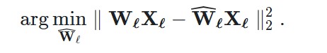
This method is inspired by a pruning technique to carefully remove weights from a fully trained dense neural network (Optimal Brain Surgeon). It uses an approximation technique and provides explicit formulas for the best single weight wqwq to remove and optimal update δFδF to adjust the set of remaining non-quantized weights FF to make up for the removal。先量化一部分,再根据误差调整没量化的部分的权重 。
GPTQ的“三步减肥法”
这个美食家的所有知识都写在一本巨大的食谱矩阵上。每一行是一道菜,每一列是一种食材。GPTQ要做的就是按列处理这本食谱。
第一步:固定顺序,统一处理(Arbitrary Order Insight)
比喻:与其在整本食谱里来回翻找最先替换的食材,GPTQ决定就从第一章的“调味料”开始,系统地处理到最后一章的“装饰品”。
第二步:懒惰批量更新(Lazy Batch-Updates)
如果每调整一列食材,就立刻重新计算整本食谱所有菜品的味道,那会累死(内存瓶颈,GPU无法高效并行)。
比喻:GPTQ不是每改一种调料就重做所有菜,而是改完一章的调料后,把这一章对整体口味的影响记下来,然后告诉下一章:“嘿,我这边咸味可能有点不够,你们后面的菜在放酱油时得多加点补回来。”
第三步:用更稳定的数学工具(Cholesky Reformulation)
当食谱巨大无比时(超大规模模型),微小的计算舍入误差会不断累积,最终可能导致“食物质变”(数值不稳定,算法崩溃)。
比喻:GPTQ聘请了一位专业的营养师(Cholesky分解),用科学的方法精确计算热量和营养补偿,确保减肥计划不会因为计算错误而搞垮美食家的身体。
总结:GPTQ的完整工作流程
# Load
 quantize config, model and tokenizer
quantize_config
 = BaseQuantizeConfig(
bits=4,
group_size=128,
damp_percent=0.01,
desc_act=False,
)
model =
 AutoGPTQForCausalLM.from_pretrained(model_id, quantize_config)
tokenizer =
 AutoTokenizer.from_pretrained(model_id)
参数详解
1. bits=4
意思:将模型权重从原始的16位(FP16)或32位(FP32)精度量化为4位整数(INT4)。
目的:这是量化的核心目标,最大程度地减小模型体积、提升推理速度。
2. group_size(组大小,即“懒惰批量”的大小)
意思:这是平衡量化质量和效率的关键参数。
工作原理:
如果不设置组大小(group_size=-1),则整个权重矩阵(比如有4096行)会共享一套量化参数(一个缩放因子)。这就像用一把尺子量整个房间,如果地面不平,误差会很大。
如果设置 group_size=1024,则会将权重矩阵分成多个小组(例如,4096行会被分成4组,每组1024行)。每个小组使用独立的量化参数。这就像用水平仪每测量1米就调整一次基准,精度更高。
注释中的评价:在实践中,设置一个组大小(尤其是 group_size=1024)能以极小的成本显著提升量化质量,是非常推荐的。
3. damp_percent(阻尼百分比)
意思:这是一个为了保证数值稳定性的技术参数。
作用:在Cholesky分解等数学计算中,为了防止因数值过小或矩阵特性不好而导致的计算失败(数值不稳定),会给矩阵的对角线元素加上一个很小的值(阻尼)。
注释中的建议:这个参数不应该被改变,除非你非常了解其背后的数学原理。使用默认值即可。
4. desc_act(激活顺序描述,也称为 act order)
意思:这是最复杂但也可能提升精度的一个参数。
工作原理:
如果 desc_act=False(默认):按固定的、连续的列顺序进行量化。
如果 desc_act=True:会先通过分析一些样本数据(输入和输出),计算每个权重列的重要性(根据其激活程度)。然后,先量化最重要的列,把量化产生的主要误差留给相对不重要的列去承担。这就像搬家时,先把易碎的贵重物品(重要权重)精心打包,剩下的普通物品(次要权重)可以打包得粗略一些。
带来的问题(权衡):
好处:通常能获得更高的量化精度。
坏处:当 desc_act=True 并且也设置了 group_size 时,由于权重被不连续地、按重要性重新排列,在推理时需要频繁地切换不同的量化参数,会导致推理速度显著下降。
注释中的决定:由于这个性能下降的问题(未来可能会修复),在当前的代码示例中选择不开启它(desc_act=False),优先保证推理速度。
The quantization process relies heavily on samples to evaluate and enhance the quality of the quantization. They provide a means of comparison between the outputs produced by the origina and the newly quantized model. The larger the number of samples provided, the greater the potential for more accurate and effective comparisons, leading to improved quantization quality. 也就是说,量化的过程取决于你提供的样本来评估精度的损失,提供的样本越多,评估越准确。
4.AWQ
保护对象不同:
量化粒度:
制定保护方案(计算缩放系数):
也就是说,GPTQ中每个group中的所有列的scale是一样的,但是AWQ每个输出通道(列)的scale不一样。